Calibration of Classification Models

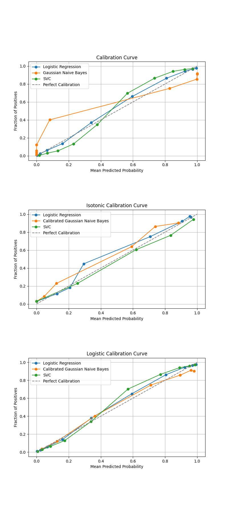
This script evaluates the calibration of multiple classification models using different calibration methods. It generates calibration curves for logistic regression, Gaussian Naive Bayes, and support vector classification (SVC), with and without calibration, and visualizes the results in a series of plots.

Logistic regression accuracy: 0.878333330154419
Gaussian naive bayes accuracy: 0.8730000257492065
Support vector classification accuracy: 0.8830000162124634
Isotonically Calibrated Logistic regression accuracy: 0.8767777681350708
Isotonically Calibrated Calibrated Gaussian naive bayes accuracy: 0.8726666569709778
Isotonically Calibrated Support vector classification accuracy: 0.8855555653572083
Logistically Calibrated Logistic regression accuracy: 0.8774444460868835
Logistically Calibrated Gaussian naive bayes accuracy: 0.8768888711929321
Logistically Calibrated Support vector classification accuracy: 0.882111132144928

import torch
import matplotlib.pyplot as plt
from sklearn.datasets import make_blobs, make_classification
from sklearn.calibration import calibration_curve as sk_calibration_curve

from DLL.Data.Metrics import calibration_curve, accuracy
from DLL.Data.Preprocessing import data_split
from DLL.MachineLearning.SupervisedLearning.LinearModels import LogisticRegression
from DLL.MachineLearning.SupervisedLearning.NaiveBayes import GaussianNaiveBayes
from DLL.MachineLearning.SupervisedLearning.SupportVectorMachines import SVC
from DLL.MachineLearning.SupervisedLearning.Kernels import Linear
from DLL.MachineLearning.SupervisedLearning.Calibration import CalibratedClassifier

# X, y = make_blobs(n_samples=100_000, n_features=2, centers=2, cluster_std=5)
X, y = make_classification(n_samples=10_000, n_features=20, n_informative=2, n_redundant=10, random_state=42)
X, y = torch.from_numpy(X).to(torch.float32), torch.from_numpy(y).to(torch.float32)
Xtrain, ytrain, _, _, Xtest, ytest = data_split(X, y, train_split=0.1, validation_split=0.0)

strategy = "quantile"



plt.figure(figsize=(8, 18))
plt.subplots_adjust(hspace=0.5)
plt.subplot(3, 1, 1)

model = LogisticRegression(learning_rate=0.01)
model.fit(Xtrain, ytrain, epochs=500)
yprob = model.predict_proba(Xtest)
print(f"Logistic regression accuracy: {accuracy(model.predict(Xtest), ytest)}")
prob_true, prob_pred = calibration_curve(ytest, yprob, n_bins=10, strategy=strategy)
plt.plot(prob_pred, prob_true, marker="o", label="Logistic Regression")

model = GaussianNaiveBayes()
model.fit(Xtrain, ytrain)
yprob = model.predict_proba(Xtest)
print(f"Gaussian naive bayes accuracy: {accuracy(model.predict(Xtest), ytest)}")
prob_true, prob_pred = calibration_curve(ytest, yprob, n_bins=10, strategy=strategy)
plt.plot(prob_pred, prob_true, marker="o", label="Gaussian Naive Bayes")

model = SVC(kernel=Linear(), opt_method="cvxopt")
model.fit(Xtrain, ytrain)
yprob = model.predict_proba(Xtest)
print(f"Support vector classification accuracy: {accuracy(model.predict(Xtest), ytest)}")
prob_true, prob_pred = calibration_curve(ytest, yprob, n_bins=10, strategy=strategy)
plt.plot(prob_pred, prob_true, marker="o", label="SVC")

plt.plot([0, 1], [0, 1], linestyle="--", color="gray", label="Perfect Calibration")
plt.xlabel("Mean Predicted Probability")
plt.ylabel("Fraction of Positives")
plt.title("Calibration Curve")
plt.legend()
plt.grid(True)


plt.subplot(3, 1, 2)

model = CalibratedClassifier(LogisticRegression(learning_rate=0.01), method="isotonic")
model.fit(Xtrain, ytrain, epochs=500)
yprob = model.predict_proba(Xtest)
print(f"Isotonically Calibrated Logistic regression accuracy: {accuracy(model.predict(Xtest), ytest)}")
prob_true, prob_pred = calibration_curve(ytest, yprob, n_bins=10, strategy=strategy)
plt.plot(prob_pred, prob_true, marker="o", label="Logistic Regression")

model = CalibratedClassifier(GaussianNaiveBayes(), method="isotonic")
model.fit(Xtrain, ytrain)
yprob = model.predict_proba(Xtest)
print(f"Isotonically Calibrated Calibrated Gaussian naive bayes accuracy: {accuracy(model.predict(Xtest), ytest)}")
prob_true, prob_pred = calibration_curve(ytest, yprob, n_bins=10, strategy=strategy)
plt.plot(prob_pred.squeeze(), prob_true.squeeze(), marker="o", label="Calibrated Gaussian Naive Bayes")

model = CalibratedClassifier(SVC(kernel=Linear(), opt_method="cvxopt"), method="isotonic")
model.fit(Xtrain, ytrain)
yprob = model.predict_proba(Xtest)
print(f"Isotonically Calibrated Support vector classification accuracy: {accuracy(model.predict(Xtest), ytest)}")
prob_true, prob_pred = calibration_curve(ytest, yprob, n_bins=10, strategy=strategy)
plt.plot(prob_pred, prob_true, marker="o", label="SVC")

plt.plot([0, 1], [0, 1], linestyle="--", color="gray", label="Perfect Calibration")
plt.xlabel("Mean Predicted Probability")
plt.ylabel("Fraction of Positives")
plt.title("Isotonic Calibration Curve")
plt.legend(loc="upper left")
plt.grid(True)


plt.subplot(3, 1, 3)

model = CalibratedClassifier(LogisticRegression(learning_rate=0.01), method="logistic")
model.fit(Xtrain, ytrain, epochs=500)
yprob = model.predict_proba(Xtest)
print(f"Logistically Calibrated Logistic regression accuracy: {accuracy(model.predict(Xtest), ytest)}")
prob_true, prob_pred = calibration_curve(ytest, yprob, n_bins=10, strategy=strategy)
plt.plot(prob_pred, prob_true, marker="o", label="Logistic Regression")

model = CalibratedClassifier(GaussianNaiveBayes(), method="logistic")
model.fit(Xtrain, ytrain)
yprob = model.predict_proba(Xtest)
print(f"Logistically Calibrated Gaussian naive bayes accuracy: {accuracy(model.predict(Xtest), ytest)}")
prob_true, prob_pred = calibration_curve(ytest, yprob, n_bins=10, strategy=strategy)
plt.plot(prob_pred.squeeze(), prob_true.squeeze(), marker="o", label="Calibrated Gaussian Naive Bayes")

model = CalibratedClassifier(SVC(kernel=Linear(), opt_method="cvxopt"), method="logistic")
model.fit(Xtrain, ytrain)
yprob = model.predict_proba(Xtest)
print(f"Logistically Calibrated Support vector classification accuracy: {accuracy(model.predict(Xtest), ytest)}")
prob_true, prob_pred = calibration_curve(ytest, yprob, n_bins=10, strategy=strategy)
plt.plot(prob_pred, prob_true, marker="o", label="SVC")

plt.plot([0, 1], [0, 1], linestyle="--", color="gray", label="Perfect Calibration")
plt.xlabel("Mean Predicted Probability")
plt.ylabel("Fraction of Positives")
plt.title("Logistic Calibration Curve")
plt.legend(loc="upper left")
plt.grid(True)

plt.show()