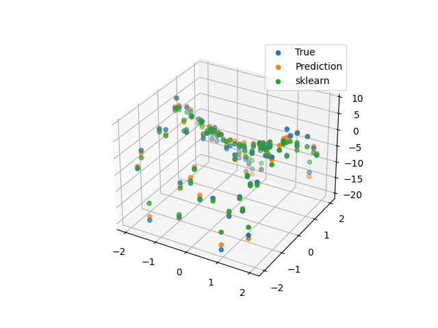
Support Vector Regression for 3D Surface Fitting

This script demonstrates the use of Support Vector Regression (SVR) to model and predict a synthetic 3D surface. The objective is to train the model to approximate the surface defined by the equation:

Z = 2 * X^2 - 5 * Y^2 + noise

The script performs the following steps:

1. Generates a synthetic 3D dataset with two input features (X, Y) and one output (Z).

2. Splits the dataset into training and test sets.

3. Trains an SVR model with a linear kernel (product of two linear kernels) and compares its predictions against a Scikit-learn SVR model with a radial basis function (RBF) kernel.

4. Visualizes the true values and the predictions from both models in a 3D scatter plot.

The comparison allows an evaluation of the model’s performance in approximating the underlying surface.

import torch
import matplotlib.pyplot as plt
from sklearn import svm

from DLL.MachineLearning.SupervisedLearning.SupportVectorMachines import SVR
from DLL.Data.Preprocessing import data_split
from DLL.MachineLearning.SupervisedLearning.Kernels import Linear


torch.manual_seed(10)

x = torch.linspace(-2, 2, 20)
y = torch.linspace(-2, 2, 20)
XX, YY = torch.meshgrid(x, y, indexing="xy")
X = XX.flatten()
Y = YY.flatten()
X_input = torch.stack((X, Y), dim=1)
Z = 2 * X ** 2 - 5 * Y ** 2 + torch.normal(0, 1, size=X.size())
x_train, y_train, x_test, y_test, _, _ = data_split(X_input, Z, train_split=0.8, validation_split=0.2)

model = SVR(kernel=Linear() ** 2)
# model = SVR()
model.fit(x_train, y_train)
y_pred = model.predict(x_test)

correct = svm.SVR(kernel="rbf", C=1)
correct.fit(x_train, y_train)
y_pred_true = correct.predict(x_test)

fig = plt.figure()
ax = fig.add_subplot(111, projection='3d')
ax.scatter(x_test[:, 0].numpy(), x_test[:, 1].numpy(), y_test.numpy(), label="True")
ax.scatter(x_test[:, 0].numpy(), x_test[:, 1].numpy(), y_pred.numpy(), label="Prediction")
ax.scatter(x_test[:, 0].numpy(), x_test[:, 1].numpy(), y_pred_true, label="sklearn")
ax.legend()
plt.show()