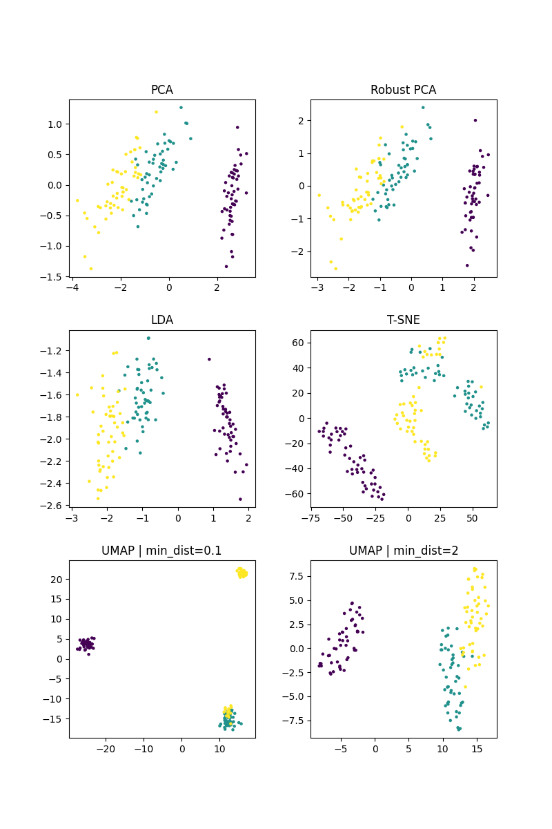
Comparison of dimensionality reduction algorithms

This script evaluates and visualizes various dimensionality reduction algorithms on the iris dataset. For each algorithm, a visualization of the latent space, which is used for comparison of the algorithms.

• 
• 

import torch
import matplotlib.pyplot as plt
from sklearn import datasets

from DLL.MachineLearning.UnsupervisedLearning.DimensionalityReduction import PCA, LDA, RobustPCA, TSNE, UMAP


# import tensorflow as tf
# (images, labels), (_, _) = tf.keras.datasets.mnist.load_data()
# X = torch.from_numpy(images).to(dtype=torch.float64).reshape(60000, -1)
# y = torch.from_numpy(labels).to(dtype=torch.int32)
iris = datasets.load_iris()
X = torch.tensor(iris.data, dtype=torch.float32)
y = torch.tensor(iris.target, dtype=torch.float32)
# X[0, 0] = 100
# X[1, 3] = 100
# breast_cancer = datasets.load_breast_cancer()
# X = torch.tensor(breast_cancer.data, dtype=torch.float32)
# y = torch.tensor(breast_cancer.target, dtype=torch.float32)

transformer_pca = PCA(n_components=2)
reduced_pca = transformer_pca.fit_transform(X, normalize=False)

transformer_UMAP1 = UMAP(n_components=2, init="spectral", p=1, n_neighbor=30, min_dist=0.1, learning_rate=1)
reduced_UMAP1 = transformer_UMAP1.fit_transform(X, epochs=300)

transformer_lda = LDA(n_components=2)
reduced_lda = transformer_lda.fit_transform(X, y)

transformer_robustPCA = RobustPCA(n_components=2, method="mcd")
reduced_robustPCA = transformer_robustPCA.fit_transform(X, epochs=10)

transformer_TSNE = TSNE(n_components=2, init="random", p=2, early_exaggeration=1, perplexity=10)
reduced_TSNE = transformer_TSNE.fit_transform(X, epochs=50)

transformer_UMAP2 = UMAP(n_components=2, init="spectral", p=1, n_neighbor=30, min_dist=2, learning_rate=1)
reduced_UMAP2 = transformer_UMAP2.fit_transform(X, epochs=300)

fig, axes = plt.subplots(3, 2, figsize=(8, 12))
plt.subplots_adjust(hspace=0.3, wspace=0.3)
axes = axes.ravel()
axes[0].scatter(reduced_pca[:, 0], reduced_pca[:, 1], c=y, s=5)
axes[0].set_title("PCA")
# axes[0].set_xlim((-5, 5))
# axes[0].set_ylim((-5, 5))
axes[1].scatter(reduced_robustPCA[:, 0], reduced_robustPCA[:, 1], c=y, s=5)
axes[1].set_title("Robust PCA")
# axes[1].set_xlim((-5, 5))
# axes[1].set_ylim((-5, 5))
axes[2].scatter(reduced_lda[:, 0], reduced_lda[:, 1], c=y, s=5)
axes[2].set_title("LDA")
axes[3].scatter(reduced_TSNE[:, 0], reduced_TSNE[:, 1], c=y, s=5)
axes[3].set_title("T-SNE")
axes[4].scatter(reduced_UMAP1[:, 0], reduced_UMAP1[:, 1], c=y, s=5)
axes[4].set_title("UMAP | min_dist=0.1")
axes[5].scatter(reduced_UMAP2[:, 0], reduced_UMAP2[:, 1], c=y, s=5)
axes[5].set_title("UMAP | min_dist=2")

plt.figure(figsize=(8, 8))
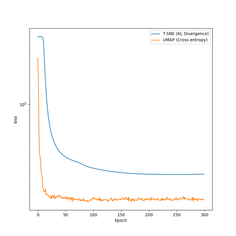
plt.semilogy(transformer_TSNE.history, label="T-SNE (KL Divergence)")
plt.semilogy(transformer_UMAP2.history, label="UMAP (Cross entropy)")
plt.xlabel("Epoch")
plt.ylabel("loss")
plt.legend()
plt.show()