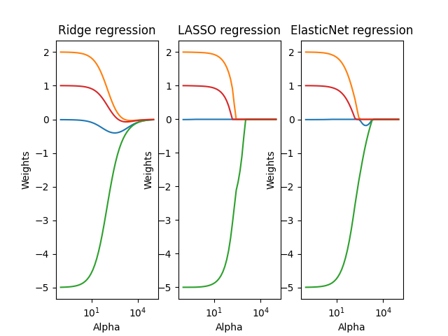
Regularization Path for Ridge, LASSO, and ElasticNet Regression

This script demonstrates the effect of L1 (LASSO), L2 (Ridge), and ElasticNet regularization on regression coefficients. It generates a 3D synthetic dataset and fits different models with varying alpha (regularization strength), tracking the weight paths.

import torch
import matplotlib.pyplot as plt
from math import log10

from DLL.MachineLearning.SupervisedLearning.LinearModels import LASSORegression, RidgeRegression, ElasticNetRegression
from DLL.DeepLearning.Optimisers import ADAM


n = 10
x1 = torch.linspace(0, 1, n)
x2 = torch.linspace(0, 1, n)
x3 = torch.linspace(0, 1, n)
XX1, XX2, XX3 = torch.meshgrid(x1, x2, x3, indexing="xy")
X = torch.stack((XX1.flatten(), XX2.flatten(), XX3.flatten()), dim=1)
y = 2 * XX1.flatten() - 5 * XX2.flatten() + 1 * XX3.flatten() + 0.1 * torch.normal(0, 1, size=XX1.flatten().size())

weights = []
alphas = torch.logspace(log10(1e-1), log10(1e5), 50).tolist()
for alpha in alphas:
    model = RidgeRegression(alpha=alpha)
    model.fit(X, y)
    weights.append(model.beta.tolist())

weights = torch.tensor(weights)

fig, axes = plt.subplots(1, 3)

for row in weights.T:
    axes[0].semilogx(alphas, row)
axes[0].set_title("Ridge regression")
axes[0].set_xlabel("Alpha")
axes[0].set_ylabel("Weights")

weights_lasso = []
weight_elasticnet = []
for alpha in alphas:
    model = LASSORegression(alpha=alpha)
    model.fit(X, y, epochs=50)
    weights_lasso.append([model.weights.tolist()])
    model = ElasticNetRegression(alpha=alpha, l1_ratio=0.5)
    model.fit(X, y, epochs=50)
    weight_elasticnet.append([model.weights.tolist()])

weights_lasso = torch.tensor(weights_lasso).squeeze()
weight_elasticnet = torch.tensor(weight_elasticnet).squeeze()

for row in weights_lasso.T:
    axes[1].semilogx(alphas, row)
axes[1].set_title("LASSO regression")
axes[1].set_xlabel("Alpha")
axes[1].set_ylabel("Weights")

for row in weight_elasticnet.T:
    axes[2].semilogx(alphas, row)
axes[2].set_title("ElasticNet regression")
axes[2].set_xlabel("Alpha")
axes[2].set_ylabel("Weights")
plt.show()