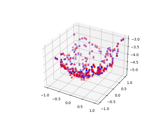
Polynomial Surface Regression with Total Least Squares

This script demonstrates polynomial regression on a 2D dataset using total least squares (TLS). It generates a grid of input points, applies polynomial feature expansion, and fits a linear regression model. Predictions are visualized in 3D, comparing model output (blue) against actual values (red).

import torch
import matplotlib.pyplot as plt

from DLL.MachineLearning.SupervisedLearning.LinearModels import LinearRegression
from DLL.Data.Preprocessing import PolynomialFeatures, data_split


model = LinearRegression()

n = 30
X, Y = torch.meshgrid(torch.linspace(-1, 1, n, dtype=torch.float32), torch.linspace(-1, 1, n, dtype=torch.float32), indexing="xy")
x = torch.stack((X.flatten(), Y.flatten()), dim=1)
y = X.flatten() ** 2 + Y.flatten() ** 2 + 0.1 * torch.randn(size=Y.flatten().size()) - 5
x_train, y_train, x_val, y_val, x_test, y_test = data_split(x, y, train_split=0.6, validation_split=0.2)
features = PolynomialFeatures(degree=2, include_bias=True)  # Both polynomial features and linear regression must not include a bias
x_train = features.transform(x_train)

model.fit(x_train, y_train, method="tls", include_bias=False)  # Both polynomial features and linear regression must not include a bias
z = model.predict(features.transform(x_test))
fig = plt.figure()
ax = fig.add_subplot(111, projection='3d')
surf = ax.scatter(x_test[:, 0], x_test[:, 1], z, color="blue")
surf = ax.scatter(x_test[:, 0], x_test[:, 1], y_test, color="red")
plt.show()