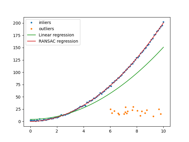
Robust Regression with RANSAC

This script demonstrates the use of RANSAC (Random Sample Consensus) regression to fit a robust model in the presence of outliers. A quadratic relationship is used to generate inlier data, while a separate set of points acts as outliers. The performance of standard linear regression is compared with RANSAC regression to highlight the latter’s robustness to noisy data.

• Inliers follow the function: ( y = 2x^2 + 1 + ext{noise} )

• Outliers are randomly distributed and do not follow the quadratic trend.

• A polynomial feature transformation is applied to the input data to allow for quadratic regression.

import torch
import matplotlib.pyplot as plt

from DLL.MachineLearning.SupervisedLearning.LinearModels import LinearRegression, RANSACRegression
from DLL.Data.Preprocessing import PolynomialFeatures


num_inliers = 100
num_outliers = 20

x_inliers = torch.linspace(0, 10, num_inliers)
y_inliers = 2 * x_inliers ** 2 + 1 + torch.randn(num_inliers)
x_outliers = torch.rand(num_outliers) * 4 + 6
y_outliers = torch.rand(num_outliers) * 20 + 10
X = PolynomialFeatures(degree=2).transform(torch.cat((x_inliers, x_outliers)).unsqueeze(-1))
y = torch.cat((y_inliers, y_outliers))
indices = torch.randperm(len(X))
X, y = X[indices], y[indices]

lr = LinearRegression()
lr.fit(X, y)
ransac = RANSACRegression(estimator=LinearRegression())
ransac.fit(X, y, min_samples=0.1)

plt.plot(x_inliers, y_inliers, ".", label="inliers")
plt.plot(x_outliers, y_outliers, ".", label="outliers")
plt.plot(x_inliers, lr.predict(PolynomialFeatures(degree=2).transform(x_inliers.unsqueeze(-1))), label="Linear regression")
plt.plot(x_inliers, ransac.predict(PolynomialFeatures(degree=2).transform(x_inliers.unsqueeze(-1))), label="RANSAC regression")
plt.legend()
plt.show()