Timeseries with SARIMA

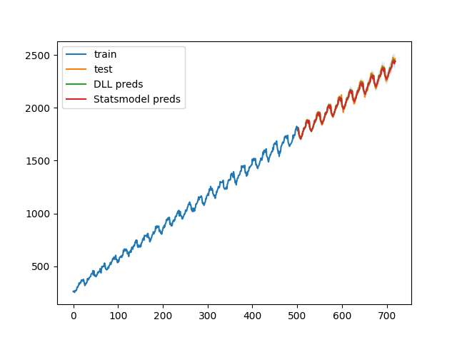
In this script, a DLL SARIMA(0, 1, 1)x(1, 1, 1, 24) model is trained and compared against a statsmodels one on a time series dataset that contains linear trend, heteroscedasticity, seasonality etc.

• 
• 
• 

import torch
import matplotlib.pyplot as plt
from statsmodels.graphics.tsaplots import plot_acf, plot_pacf
from statsmodels.tsa.statespace.sarimax import SARIMAX
import numpy as np

from DLL.MachineLearning.SupervisedLearning.LinearModels.TimeSeries import SARIMA


np.seterr(over='ignore', divide='ignore', invalid='ignore', under='ignore')  # there is some bug in DLL SARIMA, which causes numerical errors, but does not effect the fit.

n = 1000
daily = torch.tensor([9181.231, 8966.770, 8803.231, 8635.086, 8588.066, 8624.506, 8805.777, 8849.321, 9044.870, 9126.868, 9295.427, 9440.119, 9483.297, 9526.187, 9552.341, 9763.771, 10143.724, 10098.868, 10184.532, 10175.405, 10060.573, 9783.887, 10079.360, 9959.197,])
hours_per_day = 24
n_days = 30
n_hours = n_days * hours_per_day
daily_pattern = torch.tile(daily / 10, (n_days,))
torch.manual_seed(1)
series = 2 * torch.arange(n_hours) + (0.3 + torch.arange(n_hours) / n) * daily_pattern + 10 * torch.randn(n_hours)

p = 0.7
split = int(n_hours * p)
indicies = torch.arange(n_hours)
series_train = series[:split]
indicies_train = indicies[:split]
series_test = series[split:]
indicies_test = indicies[split:]

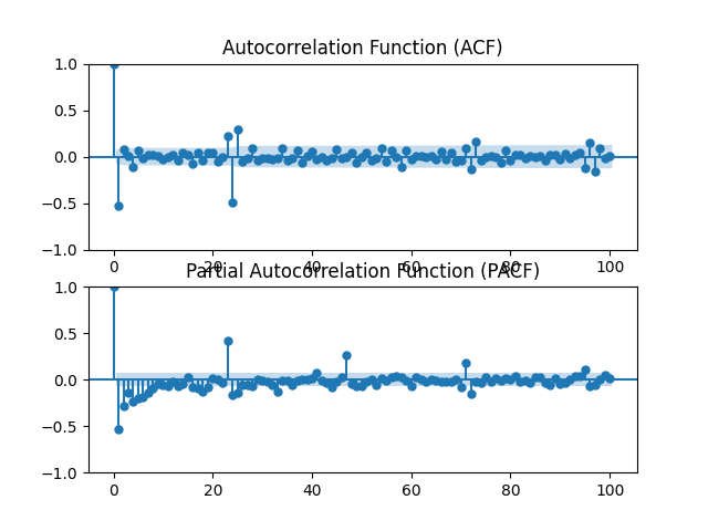
order = (0, 1, 1)  # AR(0), since no peak at pacf in the start, SAR(1), since exponentially decreasing pacf
seasonal_order = (1, 1, 1, hours_per_day)  # MA(1), since peak at 1 in acf, SMA(1), since peak at 24 in acf.
model = SARIMA(series_train, order, seasonal_order)
model.fit()
preds, upper, lower = model.predict(n_ahead=n_hours - split)
# print(model.summary())

res_sm = SARIMAX(series_train.numpy(), order=order, seasonal_order=seasonal_order, trend="n").fit(disp=False)
forecast_sm = res_sm.get_forecast(steps=n_hours - split)
y_forecast_sm = forecast_sm.predicted_mean
conf_int_sm = forecast_sm.conf_int()
# print(res_sm.summary())

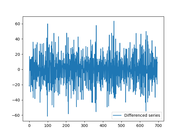
plt.figure()
diff_series = model._differentiate(series, order=order[1])
diff_series = model._differentiate(diff_series, order=seasonal_order[1], lag=hours_per_day)
plt.plot(diff_series, label="Differenced series")
plt.legend()

fig, ax = plt.subplots(2, 1)
plot_acf(diff_series.numpy(), ax=ax[0], lags=100, title="Autocorrelation Function (ACF)")
plot_pacf(diff_series.numpy(), ax=ax[1], lags=100, method="ywm", title="Partial Autocorrelation Function (PACF)")

plt.figure()
plt.plot(indicies_train, series_train, label="train")
plt.plot(indicies_test, series_test, label="test")
plt.plot(indicies_test, preds, label="DLL preds")
plt.fill_between(indicies_test, lower, upper, alpha=0.2)
plt.plot(indicies_test, y_forecast_sm, label="Statsmodel preds")
plt.fill_between(indicies_test, conf_int_sm[:, 0], conf_int_sm[:, 1], alpha=0.2)
plt.legend()
plt.show()